SOUND INTENSITY
BY BRÜEL & KJÆR
DOWNLOAD NOW
How Is Sound Intensity Measured?
The Euler Equation
Sound intensity is the time-averaged product of the pressure and particle velocity. A single microphone can measure pressure – this is not a problem. But measuring particle velocity is not as simple. The particle velocity, however, can be related to the pressure gradient (the rate at which the instantaneous pressure changes with distance) with the linearized Euler equation. With this equation, it is possible to measure this pressure gradient with two closely spaced microphones and relate it to particle velocity
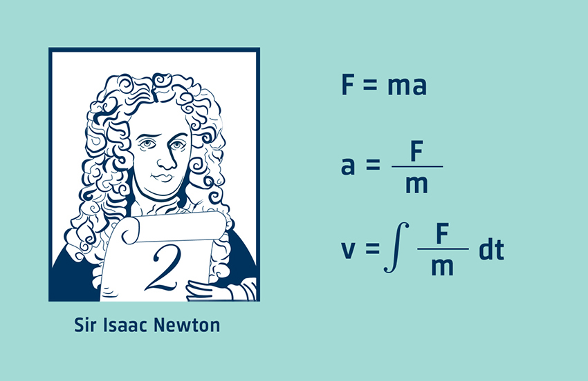
Euler’s equation is essentially Newton’s second law applied to a fluid. Newton’s second law relates the acceleration given to a mass to the force acting on it. If we know the force and the mass, we can find the acceleration and then integrate it with respect to time to find the velocity.
WHAT YOU WILL LEARN
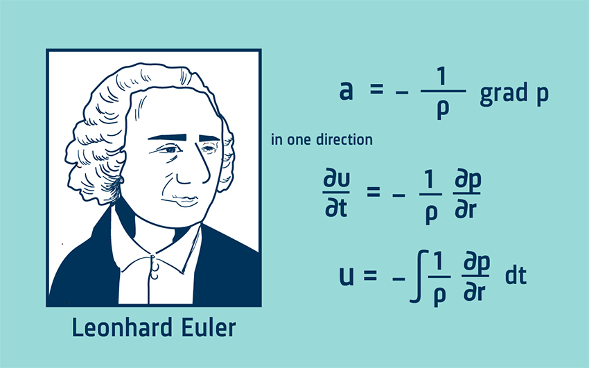
With Euler’s equation it is the pressure gradient that accelerates a fluid of density ρ. With knowledge of the pressure gradient and the density of the fluid, the particle acceleration can be calculated. Integrating the acceleration signal then gives the particle velocity.
The Finite Difference Approximation
The pressure gradient is a continuous function, that is, a smoothly changing curve. With two closely spaced microphones, it is possible to obtain a straight line approximation to the pressure gradient by taking the difference in pressure and dividing by the distance between them. This is called a finite difference approximation. It can be thought of as an attempt to draw the tangent of a circle by drawing a straight line between two points on the circumference.
The Intensity Calculation
The pressure gradient signal must now be integrated to give the particle velocity. The estimate of particle velocity is made at a position in the acoustic centre of the probe, between the two microphones. The pressure is also approximated at this point by taking the average pressure of the two microphones. The pressure and particle velocity signals are then multiplied together and time averaging gives the intensity.
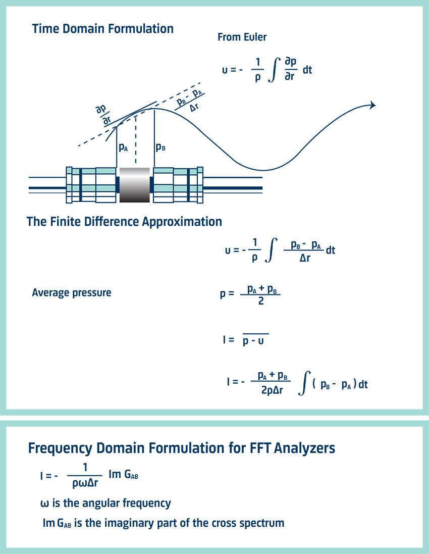
A sound intensity analyzing system consists of a probe and an analyzer. The probe simply measures the pressure at the two microphones. The analyzer does the integration and calculations necessary to find the sound intensity.
The Sound Intensity Probe
The Brüel & Kjær probe has two microphones mounted face to face with a solid spacer in between. This arrangement has been found to have better frequency response and directivity characteristics than side-by-side, back-to-back or face-to-face without solid spacer arrangements. Three solid spacers define the effective microphone separation to 6, 12 or 50 mm. The choice of spacer depends on the frequency range to be covered.
Directivity Characteristics
The directivity characteristic for the sound intensity analyzing system looks (two-dimensionally) like a figure-of-eight pattern – known as a cosine characteristic. This is due to the probe and the calculation within the analyzer.
Since pressure is a scalar quantity, a pressure transducer should have an equal response, no matter what the direction of sound incidence (that is, we need an omnidirectional characteristic). In contrast, sound intensity is a vector quantity. With a two-microphone probe, we do not measure the vector however; we measure the component in one direction, along the probe axis. The full vector is made up of three mutually perpendicular components (at 90° to each other) – one for each coordinate direction.
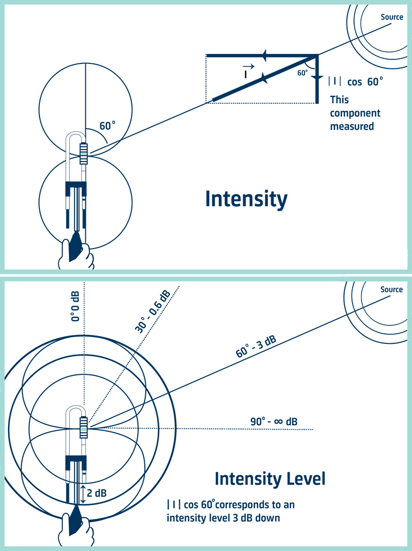
For sound incident at 90° to the axis there is no component along the probe’s axis, as there will be no difference in the pressure signals. Hence there will be zero particle velocity and zero intensity. For sound incident at an arbitrary angle θ to the axis the intensity component along the axis, will be reduced by the factor cosθ. This reduction produces the cosine directivity characteristic.
Using Sound Intensity To Determine Sound Power
The use of sound intensity rather than sound pressure to determine sound power means that measurements can be made in situ, with steady background noise and in the near field of machines. It is above all a simple technique. The sound power is the average normal intensity over a surface enclosing the source, multiplied by the surface area. First we need to define this hypothetical surface.
We can choose any enclosing surface as long as no other sources or sinks (absorbers of sound) are present within the surface. The floor is assumed to reflect all the power and so need not be included in the measuring surface. The surface may, in theory, be any distance from the source. Here are two examples:
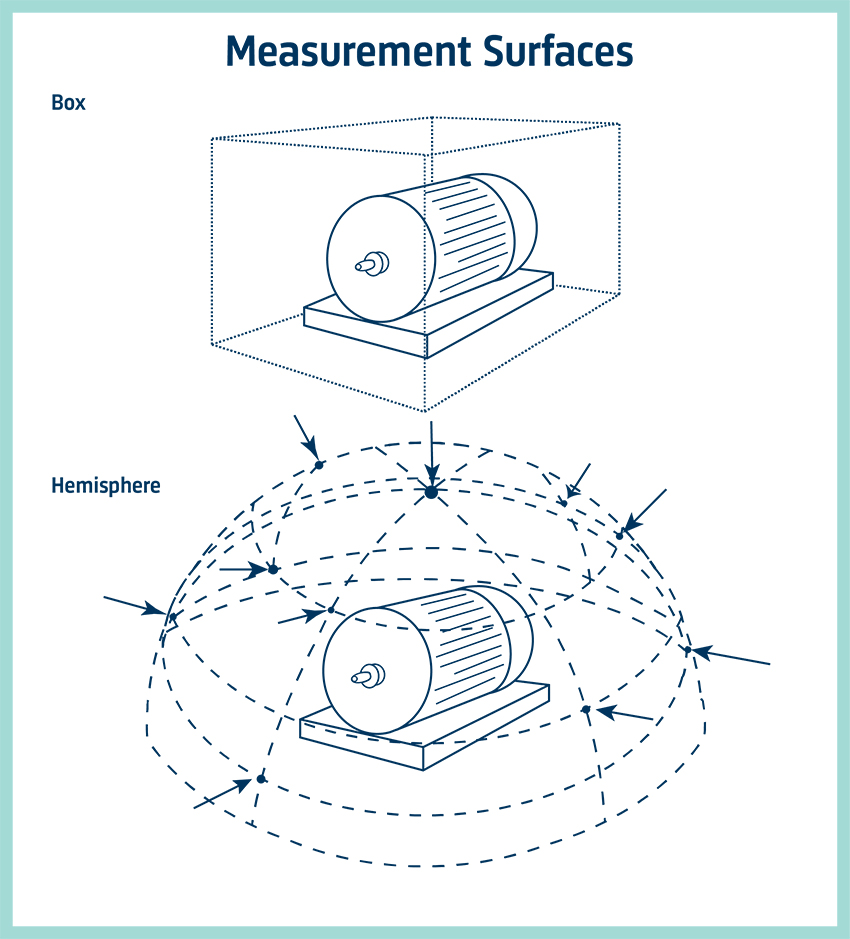
First, the box. This can be any shape and size. This surface is easy to define and the planar surfaces make averaging the intensity over the surface a simple matter. The partial sound powers can be found from each side and added.
Second, the hemisphere. This shape is most likely to give the least number of measuring points. For an omnidirectional source in the free field the intensity will be constant over a hemisphere.
Spatial Averaging
After a surface has been defined, we need to spatially average the intensity values measured normal to the surface. Note that the surface can be defined with a physical grid or just as distances from reference points. ISO 9614 contains three parts, each of which defines a different measurement method. Part 1 covers discrete point averaging and Parts 2 and 3 cover variations on swept or scanning measurements across the surface. Part 3 addresses extra requirements for measuring in a laboratory environment.
Discrete Point Averaging
In this method, the measurement surface is divided into small segments and individual measurements are made at one point per segment. The measuring points are frequently defined by a grid. This can be a frame with string or wire, although a ruler or tape measure can also be used. The results are averaged and multiplied by the surface area to find the sound power from the side.
Neither method is best for all applications and in some cases both methods may be useful. Because the swept technique is mathematically a better approximation to the continuous space integral, it is often more accurate. But care needs to be taken to sweep the probe at a constant rate and to cover the surface equally. The discrete point method, however, is often more repeatable. Both can easily be automated if repeated measurements have to be made. This also improves the accuracy.
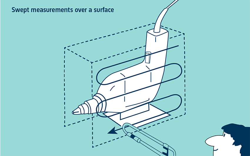
Swept Measurements over the surface
With a suitably long averaging time, the probe is simply swept over the surface, as if the surface is being painted. This gives a single-value spatial average intensity. Multiplying by the area gives the sound power from this surface. Then the sound power contributions from all the surfaces are added.