SOUND INTENSITY
BY BRÜEL & KJÆR
DOWNLOAD NOW
What about Background Noise?
One of the main advantages of the intensity method of sound power determination is that high levels of steady background noise are not important.
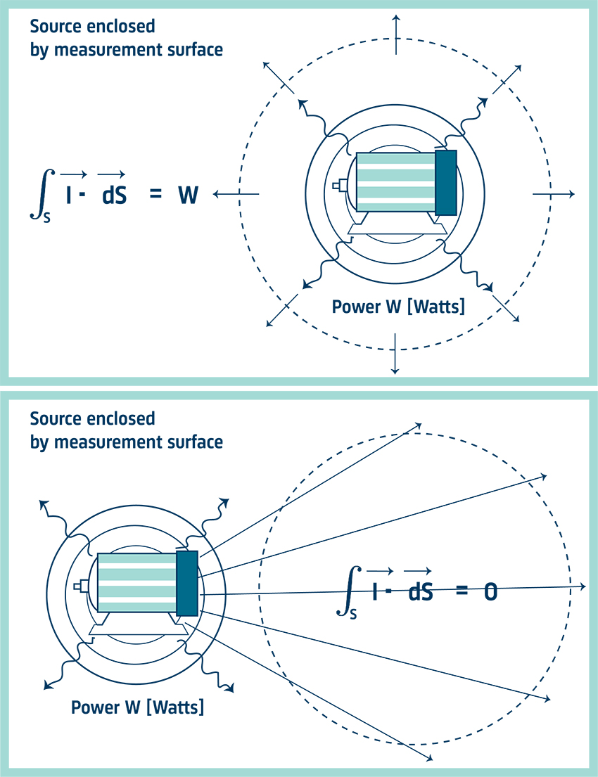
Let us imagine a surface in space – any closed volume will do. If a sound source is present within the closed surface then we can measure the average intensity over the surface of the box and multiply by the area to find the total sound power radiated by the source.
If the source were then moved outside the box and we tried to find the sound power we would measure zero. We will always measure some energy flowing in on a side. But the energy will flow out on other sides and so the contribution to the sound power radiated from the box will be zero.
WHAT YOU WILL LEARN
For this to be true, the background noise level must not vary significantly with time. If this condition is met, the noise is said to be stationary. Note, with a long enough averaging time, small random fluctuations in level will not matter. A further condition is that there must be no absorption within the box. Otherwise some background noise will not flow out of the box again.
Background noise can be regarded as noise sources outside the measurement box and will have no effect on the measured sound power of the source. In practice, this means that sound power can be measured to an accuracy of 1 dB from sources as much as 10 dB lower than the background noise. If background noise is a problem, then choosing a smaller measurement surface will improve the signal-to-noise ratio.
Intensity Mapping
Every noise control problem is first of all a problem of location and identification of the source. Sound intensity measurement offers several ways of doing this, which have considerable advantages over sound pressure measurement techniques.
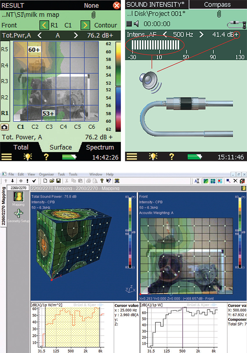
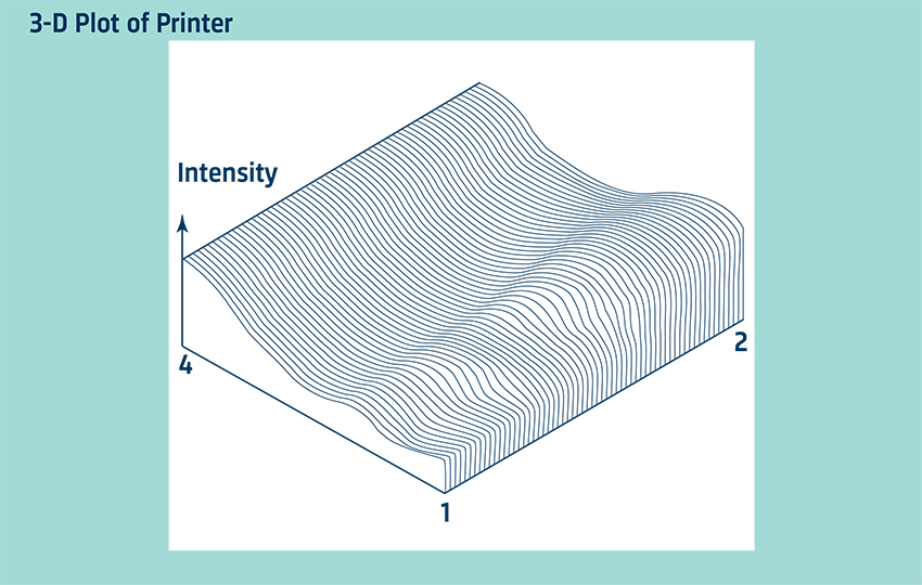
Contour Plots
Contour plots give a more detailed picture of the sound field generated by a source. Several sources and/or sinks can then be identified with accuracy.
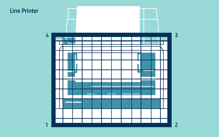
A grid is set up to define a surface. Sound intensity measurements normal to the surface are made from a number of equally spaced points on the surface. We can use the same measurements to calculate the sound power over the grid. These values are then stored. There is now a matrix of intensity levels – one value for each point. Lines of equal intensity can be drawn by interpolating and joining up points of equal intensity.
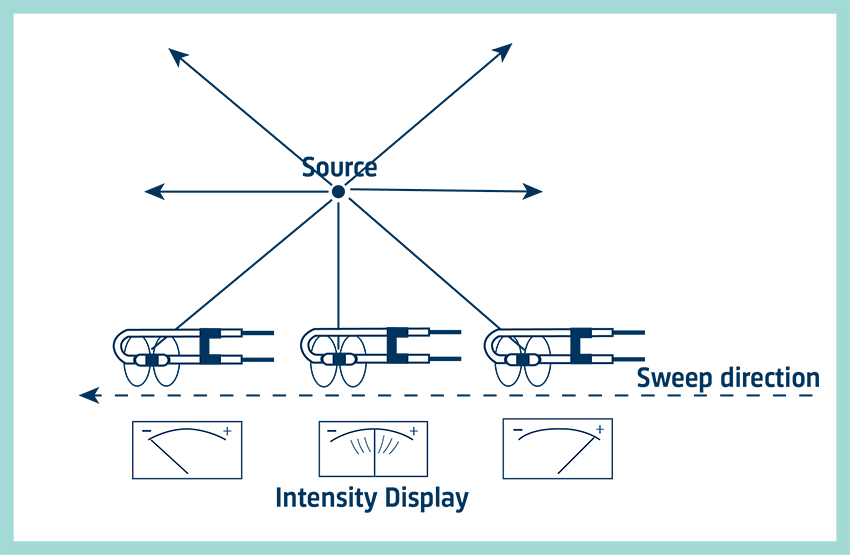
Source Location – the Null Search Method
As a quick and easy test, we can make use of the probe’s directional characteristic. Sound incident at 85° to the axis will be recorded as positivegoing intensity, whereas sound at 95° will give negative-going intensity. Therefore, there is a change in direction for only a small change in angle.
While we watch the display, the probe is swept so that its axis makes a line parallel to the plane on which we think the source is located. At some point, the direction will suddenly change. This position is identified where the display alternates rapidly between positive- and negative-going intensity. Here the sound must be incident on the probe at 90° to its axis and thus we have located the source. This method is useful when only one source is dominant – other sources or sinks may confuse the results.
Instrumentation
There are three essential components in a sound intensity analyzing system: data acquisition system, probe and calibrator. Brüel & Kjær makes a complete range of these components, as well as providing post-processing software packages, to give a choice of systems dedicated to intensity measurement.
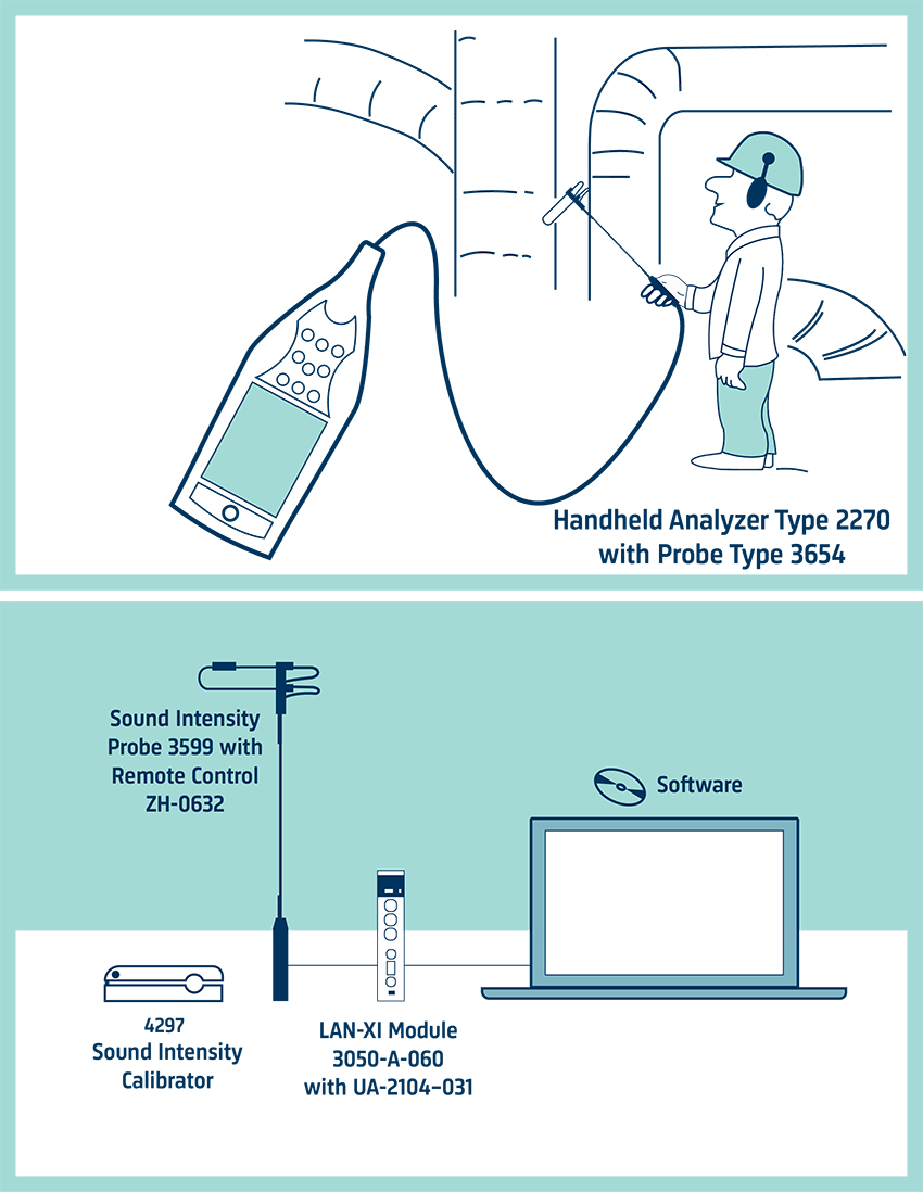
Brüel & Kjær offers sound intensity measurement solutions optimized for both laboratory and field use.
Hand-held Analyzer Type 2270, also known as the sound level meter, with Sound Intensity Software BZ-7233 is a highly portable real-time sound intensity analyzer, ideally suited to field measurements. The analyzer provides measurement guidance and workflow support for sound power determination according to ISO 9614-1, ISO 9614-2, ANSI S12.12 and ECMA 160.
PULSE™ Sound Power Using Sound Intensity Type 7882 is software for determining sound power according to ISO 9614-1, ISO 9614-2 and ISO 9614-3. Combined with Sound Intensity Probe Type 3599 and a suitable LAN-XI module, Type 7882 forms a solution ideal for sound power determination in the laboratory.
The Sound Intensity Calibrator
Type 4297 is a complete sound-intensity calibrator in one compact, portable unit with built-in sound sources. Unlike older sound intensity calibrators, Type 4297 can be used without dismantling the sound intensity probe, making it ideal for both field and laboratory use.
Making Measurements
Time Averaging
To minimize the random error, we require an averaging time long enough to give steady results. To judge the averaging time needed, several measurements can be taken and the averaging time increased until the results are repeatable.
Spatial Averaging
With swept measurements we must cover all areas equally. The sweep rate must, therefore, be constant and the area must be covered with a whole number of sweeps. With discrete point measurements, the variability in the intensity over the measuring surface determines the number of points needed. If the variability is high, the number of measuring points must be increased. It is easy to see when the spatial averaging is correct. Repeatable results for a number of different measurement surfaces, or for different measuring positions on the same surface, imply correct spatial averaging.
Background Sound
Providing the background noise is steady, measurements can be made to an accuracy of 1 dB even when the background noise measurement level exceeds the source level by as much as 10 dB. If it is possible, measuring the sound power with the source turned off (background noise on) will give an idea of the contribution of the background noise. The effect of background noise is reduced by measuring closer to the source.
Frequency Limit
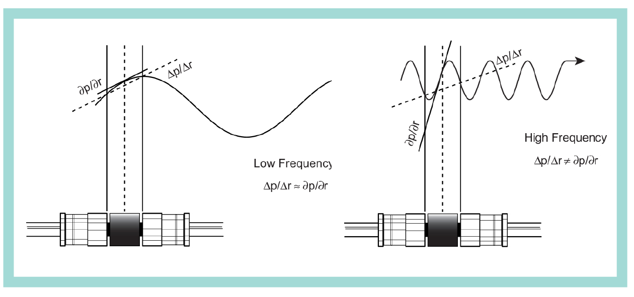
The two microphones approximate the gradient of a curve to a straight line between two points. If the curve changes too rapidly with distance, the estimate will be inaccurate. This will happen if the wavelength measured becomes small compared to the effective spacer distance.
Because it is the effective spacer distance that is compared to the wavelength, the sound intensity directional characteristics for the probe will be distorted. Most severely in the direction along the probe axis (see Figure below). For a given effective spacer distance there will be a high frequency limit beyond which errors will increase significantly. For accuracy to be within 1 dB, the wavelength measured must be greater than six times the spacer distance. This corresponds to the following high frequency limits:
- 50 mm spacer: up to 1.25 kHz
- 12 mm spacer: up to 5 kHz
- 6 mm spacer: up to 10 kHz
Extended High Frequency Limit
The face-to-face configuration of the two microphones causes resonance in the small cavity between the spacer and the membrane of the microphone. This in turn causes an increase in pressure for sound incidence along the probe axis. The pressure increase does, to some extent, compensate for distortion of the directional characteristic of the probe caused by the finite difference error.
Therefore, the operational frequency range for a Brüel & Kjær probe can be extended to an octave above the limit determined by the finite difference error if the length of the spacer between the microphones equals the diameter of the microphones, and if the levels are compensated with an optimized frequency response for the microphone pair. This phenomena was originally discovered by the authors of 'A Sound Intensity Probe for Measuring from 50 Hz to 10 kHz'; F. Jacobsen, V. Cutanda and P.M. Juhl: Brüel & Kjær Technical Review, No.1, 1996.
Low Frequency Limit
At low frequencies, there will be only a small difference between the signals from the two microphones. The measurements will therefore be more sensitive to self-generated noise and phase mismatch errors in the measurement equipment.
These problems can be reduced by using a longer spacer between the microphones, but this will reduce the high frequency limit.
The same sound signal arrives at the two microphones with a small delay that is used to calculate the velocity of the sound propagation. Because there are translations between delay, phase, and pressure-intensity index for sound intensity measurements, errors from the phase perspective can be examined and translated into the pressure-intensity index perspective.
Both the microphones and the electrical components in the measurement channels change the phase of the signals. Any difference in the change in the two channels will yield phase mismatch errors. The amount of phase mismatch between the two channels in the analyzing system determines the low frequency limit. At high frequencies, the change in phase across the spacer distance is big. For example, the phase change is 65° at 5 kHz over a 12 mm spacer. On the other hand, at low frequencies, the change in phase across the spacer distance is small. At 50 Hz, the change of phase over a 12 mm spacer is only 0.65°. For accuracy to within 1 dB, the phase change over the spacer distance should be more than five times the phase mismatch.
The international standard for sound intensity instruments IEC 61043 sets minimum requirements for the instruments, pressure-residual intensity index. These requirements can be translated into phase errors for the whole system giving ±0.086° at 50 Hz and ± 1.7° at 5 kHz.